ORB算法与源码解析
来自OpenCV
算法介绍
是ORB特征是将FAST特征点的检测方法与BRIEF特征描述子结合起来,并在它们原来的基础上做了改进与优化。
- 利用FAST特征点检测的方法来检测特征点。
- 利用Harris角点的度量方法,从FAST特征点从挑选出Harris角点响应值最大的\(N\)个特征点。
- 解决局部不变性(尺度不变性和旋转不变性),即选择从不同高斯金字塔进行检测和对特征点添加角度特征。
- 为特征点增加特征描述即描述子。
FAST检测
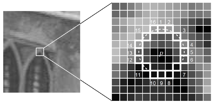
FAST特征点的检测方式即寻找一个像素点周围半径为3中的角点,如图示:
Harris评判
Harris方法是一种特征点评判方式。
其中Harris角点的响应函数定义为: \(R=det \textbf{M} - \alpha(trace\textbf{M})^2\) (其中 \(det\)指的是矩阵行列式的值;值得指的是矩阵的迹,即对角线元素之和;\(M\)指的是像素矩阵)
旋转不变性
尺度不变性的解决通过构建不同高斯金字塔(即对图像进行缩放)分别进行特征检测。而旋转不变性则是为每个特征点增加角度特征,角度的计算公式即: \(m_{pq} = \sum_{x,y}x^py^qI(x,y)\)
\[C = \left(\frac{m_{10}}{m_{00}},\frac{m_{01}}{m_{00}}\right)\] \[\theta = arctan(m_{01},m_{10})\]其中\(M_{pq}\)的定义是在以特征点为中心的一个园内,对所有像素值(以灰度为单位)以x,y坐标为权进行的加权和。即算出像素的“重心”。从而可利用公式(4)来计算出特征点的方向。
描述子计算
描述子使用BRIEF方法来进行的特征描述方式,其原理即在特征点一定邻域内按照一定的股则选取一些点对,并对这些点对的灰度值进行比较,将结果的布尔值储存下来,最终结果为长度为128/256/512长度的比特串。
下图为一些点对的选择方法:
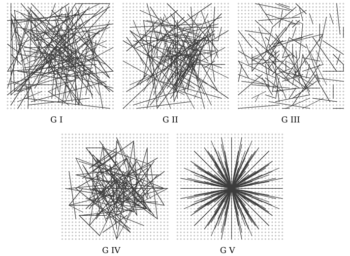
(上图分别为:1. x,y方向平均分布采样 2. x,y均服从Gauss(0,S^2/25)各向同性采样 3. x服从Gauss(0,S^2/25),y服从Gauss(0,S^2/100)采样 4. x,y从网格中随机获取 5. x一直在(0,0),y从网格中随机选取)
为了解决旋转不变性,这里选择了Steer BREIF,即在计算描述值时考虑到旋转后的结果,其公式为: \(S_{\theta} = R_{\theta}S\) 其中的\(S\)为选取的点对(\(x_n\)与\(y_n\)是一个点对两个点的灰度值),\(R_{\theta}\)为旋转不变性(公式(4))求得的旋转角度。
\[S =\begin{pmatrix}x_1&x_2&\cdots&x_{2n} \\ y_1&y_2&\cdots&y_{2n}\end{pmatrix}\] \[R_{\theta} = \begin{bmatrix} cos \theta & sin \theta \\ -sin \theta & cos \theta \end{bmatrix}\]匹配
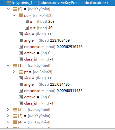
由以上几部即完成了ORB特征的提取,提取后将输出两个值,分别为关键点和描述值,其中关键点的结构如下:
class KeyPoint
{
public:
	 Point2f pt; //!< 特征点坐标
     float size; //!< 特征点描述区域大小
     float angle; //!< 特征点朝向,取[0, 360),取-1代表不可用
     float response; //!< 被选取的强度,可用于排序
     int octave; //!< 描述此点属于第几层金字塔
     int class_id; //!< 分类id,如果特征点需要被分类
};
而描述值则为Mat类型,用于储存点对。
最终匹配时跟剧描述值之间的汉明距离(即bit相同的个数)来进行比较。
代码解析
代码实现于opencv\modules\features2d\src\orb.cpp,采用OpenCV版本号为3.4.1。
FAST检测
代码833-837行,利用Fast检测方法,检测出若干潜在关键点
        // Detect FAST features, 20 is a good threshold
        {
        Ptr<FastFeatureDetector> fd = FastFeatureDetector::create(fastThreshold, true);
        fd->detect(img, keypoints, mask);
        }
Harris评价
888行,
HarrisResponses(imagePyramid, layerInfo, allKeypoints, 7, HARRIS_K);
而其具体实现在本文件131-172行
static void
HarrisResponses(const Mat& img, const std::vector<Rect>& layerinfo,
                std::vector<KeyPoint>& pts, int blockSize, float harris_k)
{
    CV_Assert( img.type() == CV_8UC1 && blockSize*blockSize <= 2048 );

    size_t ptidx, ptsize = pts.size();

    const uchar* ptr00 = img.ptr<uchar>();
    int step = (int)(img.step/img.elemSize1());
    int r = blockSize/2;

    float scale = 1.f/((1 << 2) * blockSize * 255.f);
    float scale_sq_sq = scale * scale * scale * scale;

    AutoBuffer<int> ofsbuf(blockSize*blockSize);
    int* ofs = ofsbuf;
    for( int i = 0; i < blockSize; i++ )
        for( int j = 0; j < blockSize; j++ )
            ofs[i*blockSize + j] = (int)(i*step + j);

    for( ptidx = 0; ptidx < ptsize; ptidx++ )
    {
        int x0 = cvRound(pts[ptidx].pt.x);
        int y0 = cvRound(pts[ptidx].pt.y);
        int z = pts[ptidx].octave;

        const uchar* ptr0 = ptr00 + (y0 - r + layerinfo[z].y)*step + x0 - r + layerinfo[z].x;
        int a = 0, b = 0, c = 0;

        for( int k = 0; k < blockSize*blockSize; k++ )
        {
            const uchar* ptr = ptr0 + ofs[k];
            int Ix = (ptr[1] - ptr[-1])*2 + (ptr[-step+1] - ptr[-step-1]) + (ptr[step+1] - ptr[step-1]);
            int Iy = (ptr[step] - ptr[-step])*2 + (ptr[step-1] - ptr[-step-1]) + (ptr[step+1] - ptr[-step+1]);
            a += Ix*Ix;
            b += Iy*Iy;
            c += Ix*Iy;
        }
        pts[ptidx].response = ((float)a * b - (float)c * c -
                               harris_k * ((float)a + b) * ((float)a + b))*scale_sq_sq;
    }
}
代码最后几行即为计算我们公式(1)的具体计算,其中用到了这样的公式,即在矩阵\(\textbf{M} = \begin{bmatrix} A&C \\ C&B \end{bmatrix}\)中:
\[det\textbf{M} = \lambda_1\lambda_2=AB-C^2\] \[trace\textbf{M}=\lambda_2+\lambda_2=A+B\]旋转不变性
角度的计算有下代码实现,实现在176-210行。
static void ICAngles(const Mat& img, const std::vector<Rect>& layerinfo,
                     std::vector<KeyPoint>& pts, const std::vector<int> & u_max, int half_k)
{
    int step = (int)img.step1();
    size_t ptidx, ptsize = pts.size();

    for( ptidx = 0; ptidx < ptsize; ptidx++ )
    {
        const Rect& layer = layerinfo[pts[ptidx].octave];
        const uchar* center = &img.at<uchar>(cvRound(pts[ptidx].pt.y) + layer.y, cvRound(pts[ptidx].pt.x) + layer.x);

        int m_01 = 0, m_10 = 0;

        // Treat the center line differently, v=0
        for (int u = -half_k; u <= half_k; ++u)
            m_10 += u * center[u];

        // Go line by line in the circular patch
        for (int v = 1; v <= half_k; ++v)
        {
            // Proceed over the two lines
            int v_sum = 0;
            int d = u_max[v];
            for (int u = -d; u <= d; ++u)
            {
                int val_plus = center[u + v*step], val_minus = center[u - v*step];
                v_sum += (val_plus - val_minus);
                m_10 += u * (val_plus + val_minus);
            }
            m_01 += v * v_sum;
        }

        pts[ptidx].angle = fastAtan2((float)m_01, (float)m_10);
    }
}
计算描述子
实现在214行到415行,摘取重要部分:
static void
computeOrbDescriptors( const Mat& imagePyramid, const std::vector<Rect>& layerInfo,
                       const std::vector<float>& layerScale, std::vector<KeyPoint>& keypoints,
                       Mat& descriptors, const std::vector<Point>& _pattern, int dsize, int wta_k )
{
// ...
    //矩阵相乘
    #define GET_VALUE(idx) \
               (x = pattern[idx].x*a - pattern[idx].y*b, \
                y = pattern[idx].x*b + pattern[idx].y*a, \
                ix = cvRound(x), \
                iy = cvRound(y), \
                *(center + iy*step + ix) )
    //...
    //实现公式(5)
    for (i = 0; i < dsize; ++i, pattern += 16)
    {
        int t0, t1, val;
        t0 = GET_VALUE(0); t1 = GET_VALUE(1);
        val = t0 < t1;
        t0 = GET_VALUE(2); t1 = GET_VALUE(3);
        val |= (t0 < t1) << 1;
        t0 = GET_VALUE(4); t1 = GET_VALUE(5);
        val |= (t0 < t1) << 2;
        t0 = GET_VALUE(6); t1 = GET_VALUE(7);
        val |= (t0 < t1) << 3;
        t0 = GET_VALUE(8); t1 = GET_VALUE(9);
        val |= (t0 < t1) << 4;
        t0 = GET_VALUE(10); t1 = GET_VALUE(11);
        val |= (t0 < t1) << 5;
        t0 = GET_VALUE(12); t1 = GET_VALUE(13);
        val |= (t0 < t1) << 6;
        t0 = GET_VALUE(14); t1 = GET_VALUE(15);
        val |= (t0 < t1) << 7;

        desc[i] = (uchar)val;
    }
    //...
}
代码运行时数据
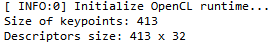
在运行时,选取的特征描述子是256bit的,即32个unsigned char的大小,可以由下图的运行数据大小得知:
运行后的数据:
部分关键点及其数据:
对应的描述子:

(三十二个为一个描述子,图中并未截全一个描述子)
您可能需要科学上网来加载评论框